

Data pipeline bottlenecks rarely announce themselves. A dashboard refreshes an hour late, a nightly job overruns its window, or a queue grows every Monday, and teams start guessing. Because one slow stage can hide behind a long chain of dependencies, guessing often ends in bigger clusters and higher bills without a real fix.
A data pipeline bottleneck is any stage where limited capacity, inefficient design, or contention slows the entire flow of data. The constraint may sit in the source system, network, compute layer, storage, database, or orchestration layer. The slowest stage sets the pace for everything after it, so one constrained step raises latency, delays downstream jobs, and lowers overall efficiency.
The first step is not to add more infrastructure. It is to find out where the pipeline spends its time and why, because in a surprising number of cases, more compute will not fix the problem. Keep that principle in mind as you read: it comes up again in the ingestion and database sections below, where it matters most.
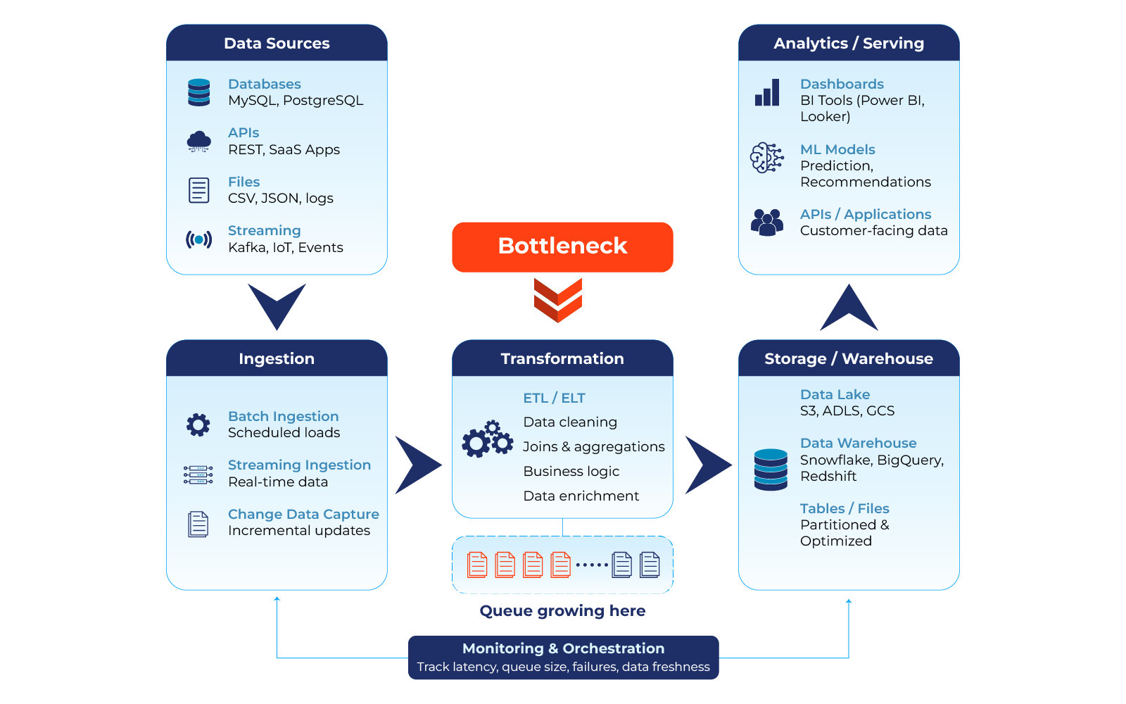
Why Bottlenecks Matter
Left unresolved, bottlenecks cost more than run time: stale dashboards, late ML features and customer-facing data, higher compute spend from reruns, and engineering time spent firefighting instead of building. Warning signs include batch windows that keep growing, consumer lag that never clears, jobs that finish late only on heavy-volume days, and compute costs rising faster than data volume.
Where Bottlenecks Come From
Most constraints trace back to growth. Designs that worked at small scale, full reloads, one long serial workflow, break as volume, consumers, and schema changes pile up. A pipeline can also look healthy at one stage while waiting at another: an ETL job may have plenty of compute but spend most of its runtime waiting on a source API, or a Spark job may have enough executors but stay slow because one partition holds a disproportionate share of the data.
Before troubleshooting, establish a baseline for: end-to-end latency, records or bytes processed, backlog size, stage-level runtime, error and retry rates, and data freshness. This baseline is what separates a genuine bottleneck from a normal increase in workload.
Bottlenecks at a Glance
| Stage | Common signal | Practical response |
|---|---|---|
| Ingestion | Growing backlog, incomplete loads | Incremental loads, batching, controlled concurrency |
| Transformation | Long-running tasks, OOM errors | Profile code, reduce repeated work |
| Partitioning | Uneven task duration | Rebalance keys or partitions |
| Database | Query time dominates | Tune queries, writes, and partitions |
| Storage | Many small files, high scan cost | Compact files, adjust batch size |
| Network / I/O | High wait time | Reduce data movement, optimize transfer |
| Orchestration | Idle compute, missed windows | Parallelize independent tasks |
| Serving | Slow dashboards | Optimize queries, pre-aggregate |
1. Slow or Constrained Ingestion
Ingestion is often the first bottleneck, especially with APIs, operational databases, or third-party platforms, the limit usually sits in the source, not the pipeline code, so code reviews tend to miss it. Common causes: API rate limits, single-threaded extraction, small batches, connection limits, repeated full-table loads, and unannounced schema changes that break parsing.
Symptoms: the input backlog keeps growing, source requests spend most of their time waiting, downstream workers sit idle and retries spike during peak periods.
Example. A team ingests order data from a marketplace API every few minutes and, when the pipeline falls behind, doubles the size of the Spark cluster pulling the data. Throughput does not improve, because the API still only allows a fixed number of requests per minute, the cluster was never the constraint. This is the clearest version of a rule worth remembering: more compute only helps when compute is the limit.
Fixes: incremental loads or change data capture (CDC) so only new and changed records move; read from a replica so extraction never competes with production traffic; split large extracts in parallel by key or date range; use pagination, checkpointing, and connection reuse; buffer bursts in a queue; and validate schemas at ingestion so upstream changes fail fast instead of silently.
2. Expensive Transformations
Transformation stages become bottlenecks when they compute more than the result needs. This is especially visible in ETL jobs, where join design and partition handling set the pace. Common causes: large joins and aggregations, repeated scans, row-by-row logic, expensive UDFs, unnecessary serialization, and reprocessing full history when only a few partitions changed.
Example. A reporting job joins billions of transaction records with customer and product tables even though the report only covers the last 30 days. Pushing the date filter before the join, instead of after, can cut the data volume the join has to handle by an order of magnitude.
Fixes: filter and select only needed columns before joining; reprocess only the affected partitions on late-arriving data; replace row-by-row logic with set-based operations; size compute from measured peaks rather than guesswork; and, where it fits, load first and transform inside the warehouse (ELT) instead of transforming in-flight.
3. Data Skew and Partitioning
Partitioning lets distributed systems divide work across workers. Poor partitioning does the opposite: one worker gets most of the data while the rest sit idle. Skew usually comes from a hot key (a handful of customers or products that dwarf everyone else) or a placeholder key (a null or “unknown” ID that silently collects every unmatched row).
Example. In the Spark UI, a stage shows 199 tasks finishing in under a minute and one task still running twenty minutes later, the classic signature of skew. The long task is usually the partition holding a hot key or the “unknown” placeholder. The same pattern shows up as a single reducer straggling behind the rest of a shuffle.
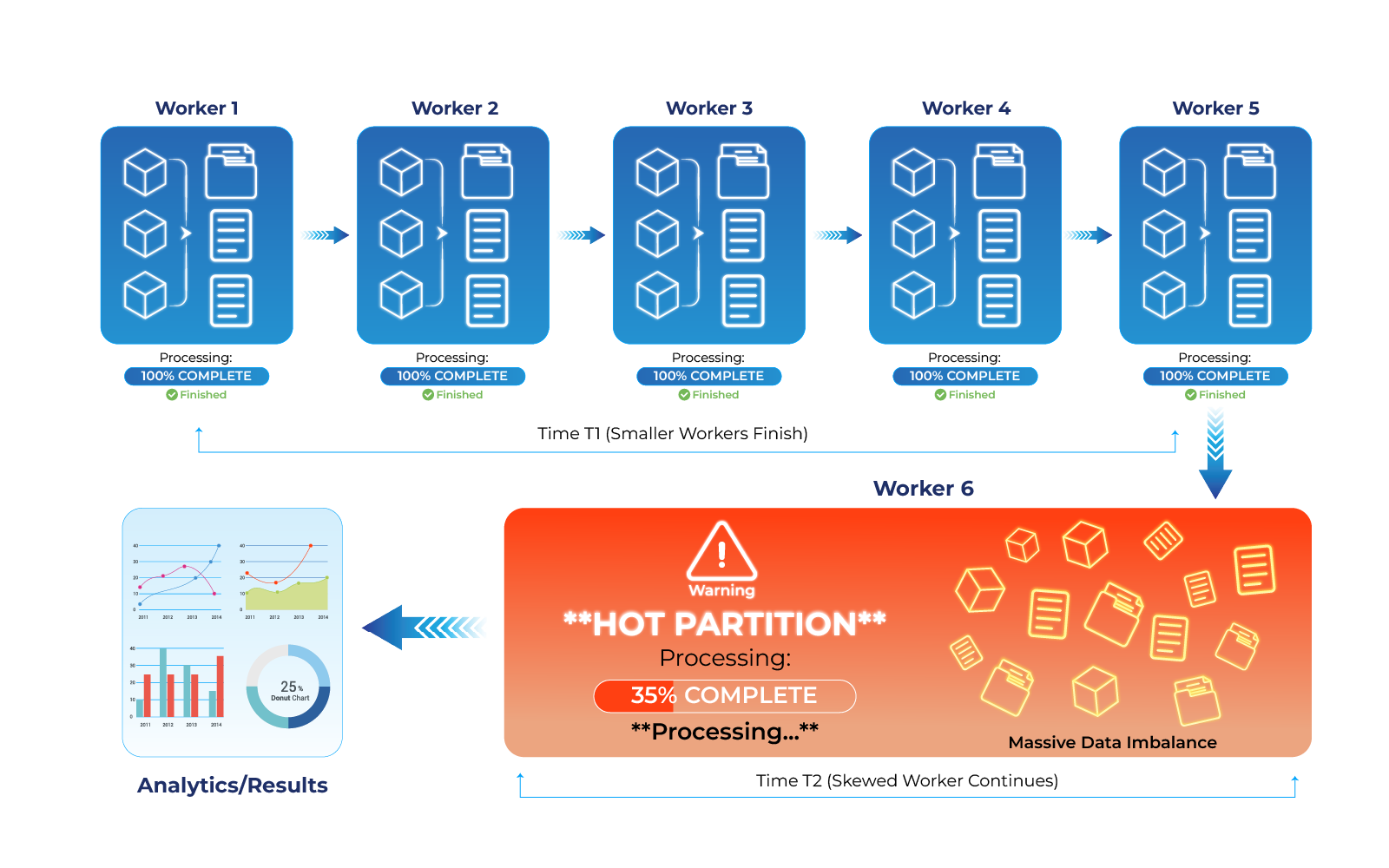
Fixes: isolate placeholder keys before the join; choose a more balanced partition key; salt hot keys (append a random suffix to spread them across partitions); broadcast small tables to avoid a large shuffle; and pre-aggregate before the expensive step. More workers will not fix this, the data itself is unevenly distributed, and extra capacity just gives the idle workers more time to wait.
4. Database and Warehouse Constraints
A pipeline can look like a transformation problem when the real constraint is the destination database or warehouse: large table scans, inefficient joins, poor query plans, excessive concurrency, or unbatched writes.
Example. A daily load spends three minutes moving data and thirty minutes running a warehouse-side MERGE against a large historical table. Adding bandwidth does nothing here, because the bottleneck is the query plan, not the transfer.
Shared warehouses add a scheduling version of the same problem: a nightly load that overruns into the morning forces analyst queries to compete with the load for the same resources. Resource pools that separate heavy jobs from time-critical ones, plus running independent models in parallel, keep the morning peak clear. When diagnosing, separate data movement time from processing time — checking the query plan, scan volume, and concurrency will point to the real constraint faster than adding resources will.
5. Small Files and Fragmented Storage
File-based pipelines slow down when they generate thousands of very small files, usually from frequent micro-batches or overly granular partitioning. The engine spends its time opening and coordinating files rather than processing data.
Example. A Delta Lake table fed by frequent small streaming writes accumulates thousands of tiny Parquet files. Queries against it slow down and scan costs climb even though the total data volume has not changed much. The table may benefit from OPTIMIZE (file compaction) or another file-management strategy, depending on the platform and workload, rather than simply increasing cluster size.
Fixes: buffer writes into larger batches where latency allows; schedule regular compaction; partition by common filter columns such as date, without going too granular; and separate frequently updated data from historical data. The right file size depends on the engine, so measure rather than apply a universal threshold.
6. Network and Data-Location Constraints
A pipeline can have plenty of compute and still be slow because it spends most of its time waiting for data. Cross-region transfers, slow storage, remote databases, and repeated movement between environments all add I/O latency. For example, extracting in one region, processing in another, and writing to a third storage layer, where each step is individually fast but the transfers dominate total runtime. Where the architecture allows it, keep frequently exchanged data closer together, and use compression when the added CPU cost is worth the reduced transfer volume.
7. Orchestration and Dependency Delays
Not every bottleneck is computational. Pipelines also lose time waiting on other tasks. Long dependency chains, unnecessary sequential execution, and poor failure handling all add latency.
Example. Five independent extraction jobs run one after another, so total runtime is the sum of all five. Running them concurrently instead cuts wall-clock time without touching the underlying logic, but concurrency should be bounded, since running everything at once can overload a shared API or database.
A related trap: fixed retry intervals against a rate-limited API can trigger a retry storm, where a failing task floods the system with repeated attempts and crowds out the calls that would have succeeded. Exponential backoff avoids this.
8. Weak Monitoring
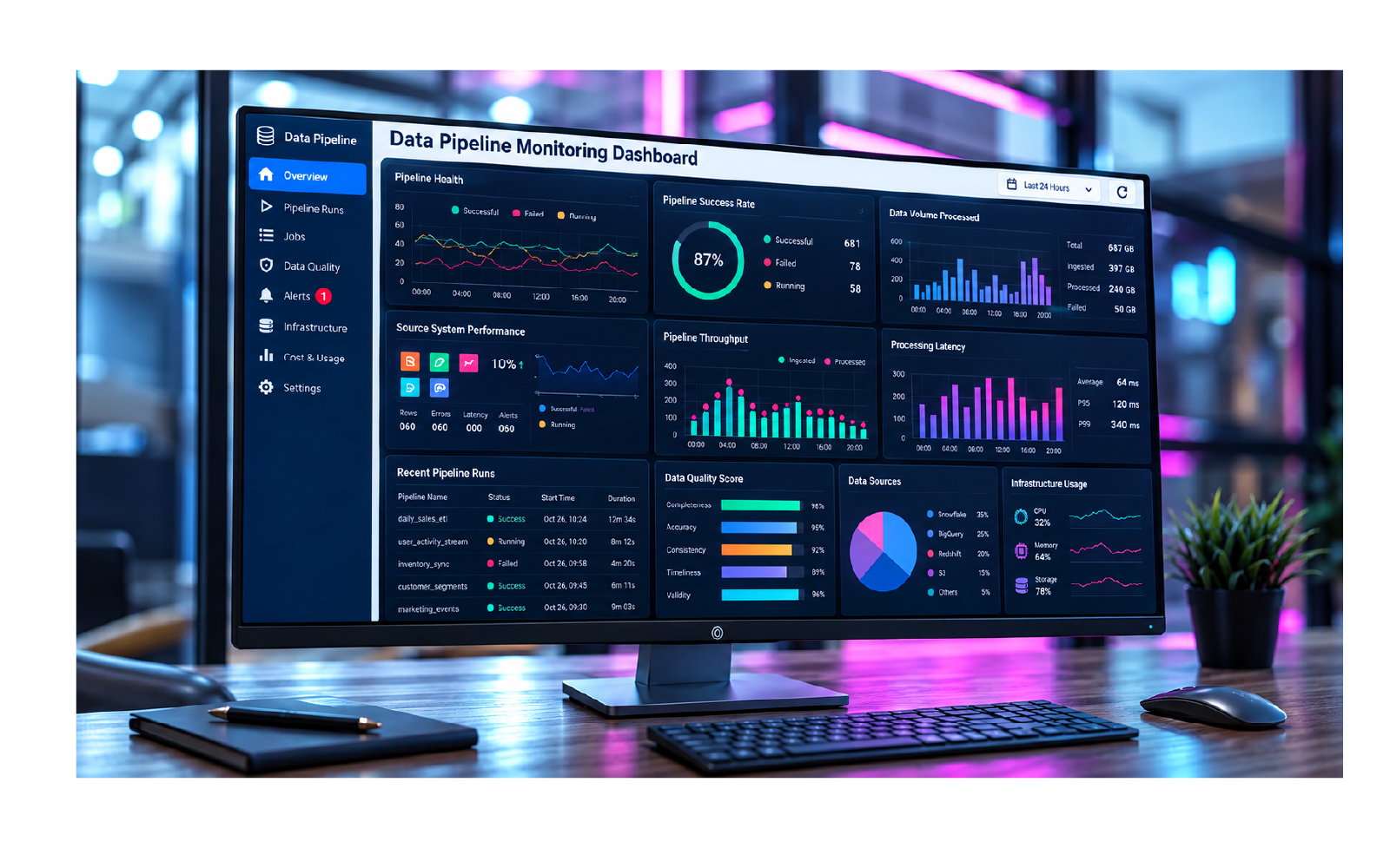
A pipeline that reports “success” is not necessarily healthy, a job can finish while delivering data hours late or processing far fewer records than expected. Observability (understanding the system from logs, metrics, and traces) turns the following into alerts and trend lines:
| Metric | What it reveals | Warning sign |
|---|---|---|
| Stage duration | Slowest step | Steady upward trend |
| Throughput | Processing capacity | Flat while volume grows |
| Queue depth / lag | Ingestion backlog | Growing lag |
| Task skew | Uneven work | One task far above the median |
| Resource use | Over/under-provisioning | Mixed CPU or long idle |
| Retry rate | Reliability | Rising retries |
| Data freshness | Delivery delay | Data older than its target |
Use percentile metrics such as p95 run time, they surface outliers that averages hide. If a pipeline that normally processes 50 million records in 20 minutes suddenly takes 50 minutes for the same volume, job success alone won’t reveal why; stage-level metrics will.
How to Troubleshoot a Slow Pipeline
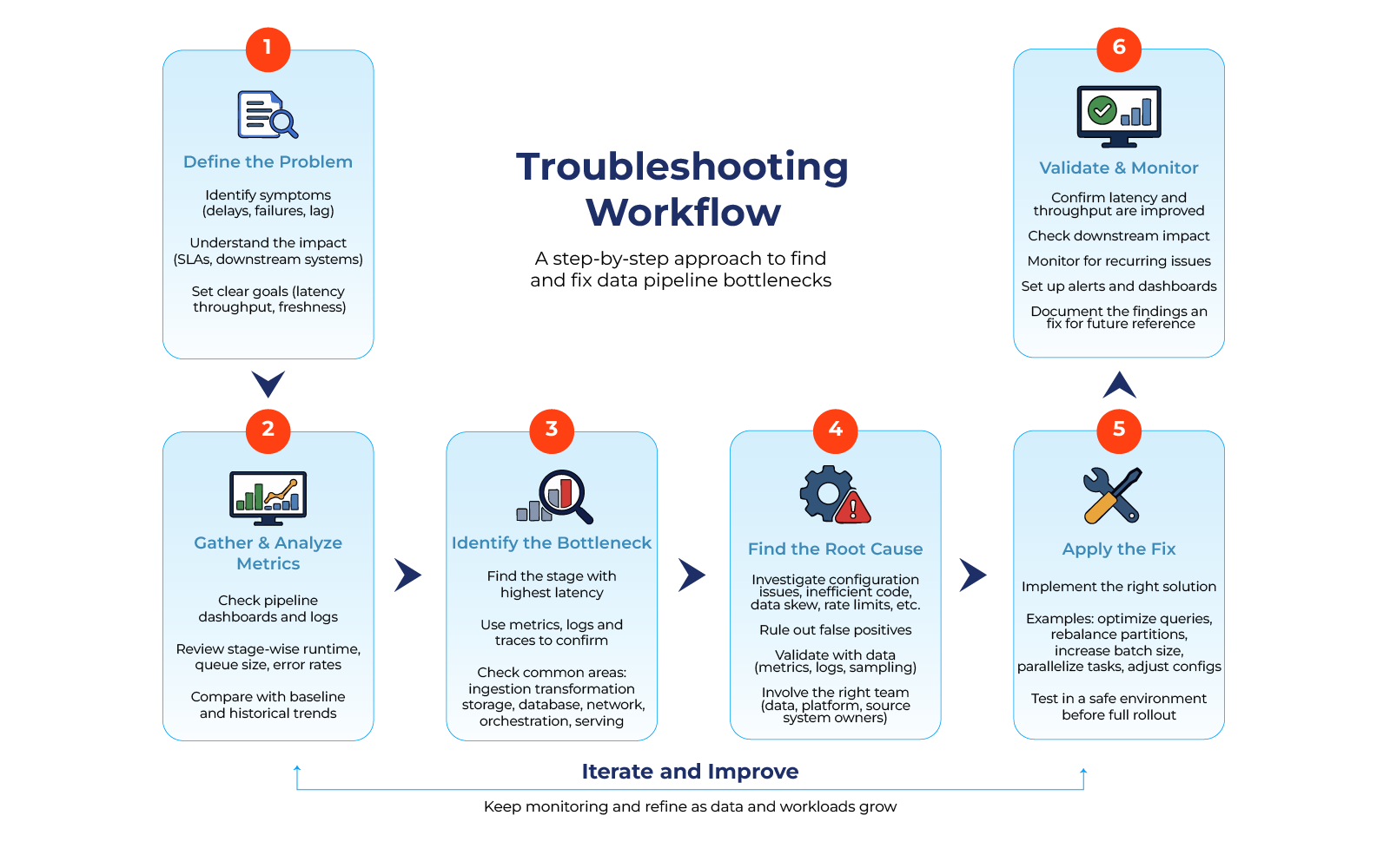
A structured investigation beats changing several settings at once:
- Establish a baseline. Compare the slow run against a healthy run of similar volume.
- Locate the constrained stage. Trace source to destination and find the critical path, the longest chain of dependent tasks.
- Compare duration with volume. Non-linear growth (runtime doubling while volume rises 20%) points to skew, spills, or contention.
- Isolate the wait. Separate CPU, memory, network, storage, database, and scheduling time.
- Check the distribution of work. For distributed jobs, compare partition sizes and task durations; one long task can delay an otherwise finished stage.
- Test one variable at a time. Batch size, partitioning, query logic, or concurrency, and re-measure against the baseline.
Validate the data. A faster run only counts if the output is still complete, accurate, and deduplicated.
Real-World Scenarios
| Scenario | Symptom | Root cause | Fix |
|---|---|---|---|
| Retail nightly ETL | Load grows from 3h to 6h while volume only doubles | Join skew on an "unknown" customer key | Isolate the placeholder key, salt hot keys, compact files |
| Streaming to a data lake | Reads slow, scan costs climb | Thousands of tiny files per hour | Buffer writes into larger files, schedule compaction |
| SaaS API ingestion | Loads miss the window, retries pile up | Rate limits + fixed retry intervals | Pull only changed records, retry with backoff |
| Shared warehouse | Morning dashboards slow | Nightly models overrun into analyst hours | Separate resource pools, parallelize models |
| Upstream schema change | Jobs fail overnight, reruns pile up | Unannounced column changes | Validate schemas at ingestion, quarantine bad records |
In the retail case, stage timings showed the join step consuming most of the runtime, with one key holding a large share of all rows. After the fixes, the job finished well before its 6 a.m. deadline, and an alert now fires whenever a stage exceeds its baseline by 20%.
Worked Example: The Hidden Skew
An e-commerce pipeline runs Ingestion → Product enrichment → Sales aggregation → Warehouse load. Ingestion and enrichment finish on time, but aggregation develops a growing backlog. The Spark UI shows one task running far longer than the rest, a handful of high-volume products have created a hot partition under product ID. The team repartitions and salts the hot key instead of adding workers; the stage drops from roughly two hours to under thirty minutes, and the backlog clears. The visible symptom was slow processing; the real bottleneck was workload distribution.
| Symptom | Likely bottleneck | First check |
|---|---|---|
| Backlog grows | Source or ingestion | Source latency, rate limits, batch size |
| One worker runs much longer | Skew or partitioning | Records and duration by partition |
| Database step dominates | Query or write path | Query plan, scans, concurrency |
| Workers mostly idle | Dependency or I/O wait | Stage timing and wait metrics |
| Runtime rises with file count | File layout | File size and partition count |
| Jobs succeed but data is late | Scheduling or upstream delay | Freshness and dependency timing |
Optimizing: A Practical Order of Work
Start with low-effort changes and move to redesign only once measurements justify it. Quick wins: column pruning, early filtering, file compaction. Higher effort, higher ceiling: incremental modeling and repartitioning.
Checklist
- Define latency and throughput targets, and baseline cost per stage
- Compare slow runs against normal runs
- Replace full reloads with incremental loads
- Profile expensive transformations and review partition and file layout
- Examine database query plans
- Parallelize independent tasks and tune retries/backoff
- Set alerts on duration, lag, and failure rate
- Validate data quality after every change
Mistakes to Avoid
- Scaling up before locating the constraint, raises cost and hides the real design flaw
- Tuning for the average day instead of the worst day
- Changing several settings at once, hides which change worked
- Dropping validation checks for speed, risks data quality
Designing for Scalability
Scalability is different from performance: performance is how fast the pipeline runs today; scalability is whether that speed holds as volume, sources, and users grow. A pipeline that handles 10 million records comfortably can behave very differently at 100 million if the source, database, or orchestration layer has a fixed limit.
Scalable pipelines tend to share a few habits: incremental processing; partition-aware storage; horizontal scaling (more workers, not just bigger machines) where compute genuinely is the constraint; decoupled stages via queues or storage layers, so one slow step cannot block the rest; bounded concurrency; idempotent tasks and writes, so reruns never duplicate data; and automated monitoring. Load test with projected volume and revisit capacity each quarter, evaluated across the whole pipeline, not just the compute layer.
Conclusion
Data pipeline bottlenecks rarely come from one dramatic failure. They build slowly through growing volume, uneven data, and designs that no longer fit. Measure each stage, find the critical path, fix the true constraint, and confirm the result, and remember the thread running through every section above: a rate-limited API, a skewed partition, an inefficient warehouse query, or a small-file problem will keep constraining performance no matter how much compute you throw at it.
If you’d like an outside view on your architecture, RDSolutions can help audit your pipelines, pinpoint the constrained stage, and plan the fixes that matter most.
Frequently Asked Questions
A data pipeline bottleneck is a stage that limits the overall rate at which data can be processed or delivered. It can result from limited capacity or inefficient design, such as slow source extraction, skewed joins, small files, or serial dependencies.
Teams can identify bottlenecks by measuring runtime for each stage, finding the critical path, and comparing duration with input volume. The slowest stage should then be checked for CPU, memory, disk, network, and partition skew.
Common causes include API rate limits, slow source systems, small batches, connection limits, and repeated full-load extraction. Incremental extraction, batching, checkpointing, and controlled concurrency can help reduce these constraints.
No. Additional compute helps when processing capacity is the limiting factor. It will not solve problems caused by API rate limits, database constraints, partition skew, or serialized dependencies, and may increase cost without reducing runtime.
Key metrics include stage duration, throughput, queue lag, task skew, resource utilization, retry rate, and data freshness. Together, these signals help identify where constraints form and whether pipeline performance is getting worse.
Pipelines should be monitored continuously using dashboards and alerts, with a deeper performance review performed periodically, such as each quarter or after major changes in data volume, schema, workload, or architecture.

Saurabh Tikekar | Data Engineer
Tired of broken scrapers and messy data?
Let us handle the complexity while you focus on insights.